Energy-Aware Wind-Resilient Routing for Truck-Assisted Multi-UAV Delivery under Wind Uncertainty

1. The Dynamic Wind Hazard: Why Deterministic UAV Routing Fails

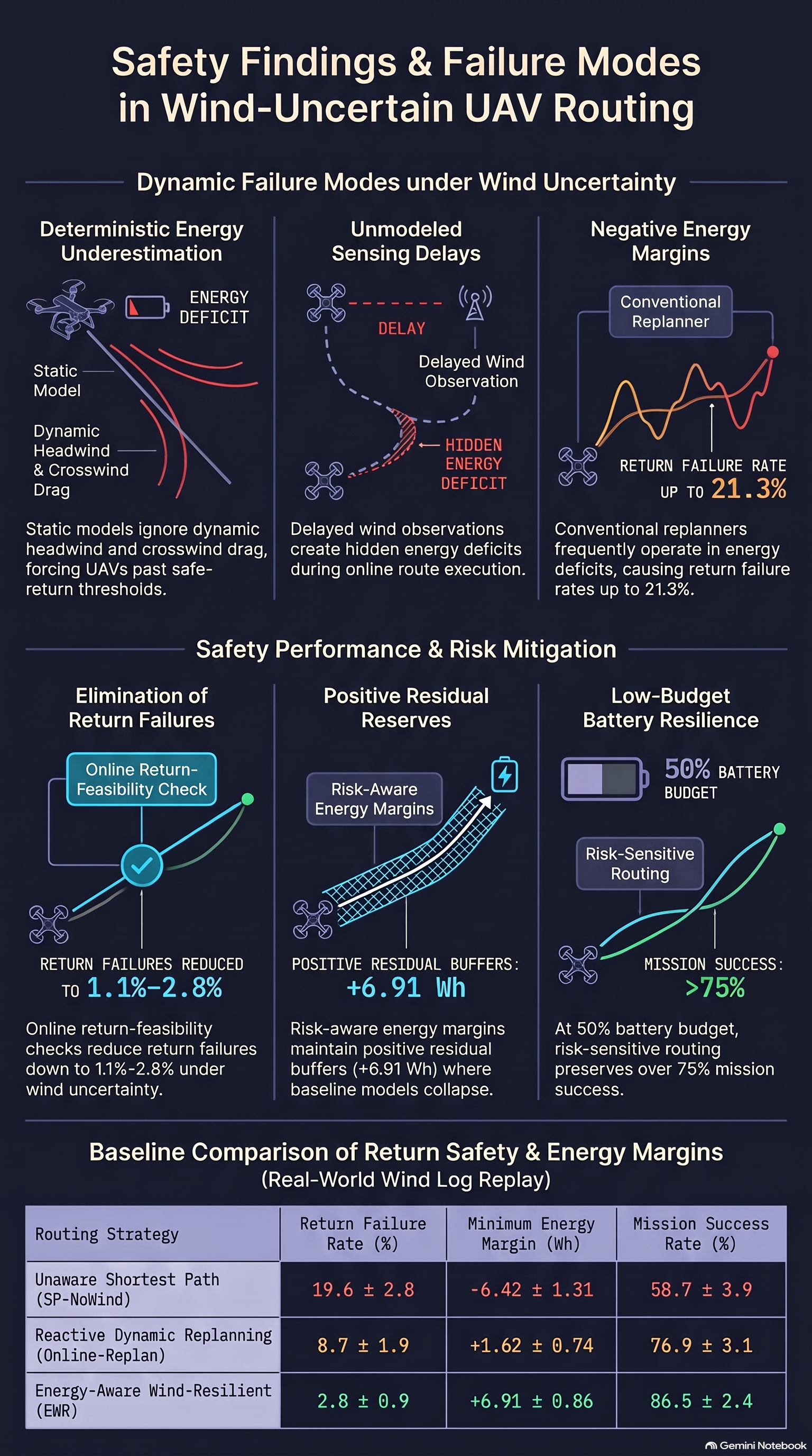
In air-ground autonomous delivery systems, mobile ground vehicles provide long-range transport and payload capacity, while unmanned aerial vehicles (UAVs) are deployed from the vehicle platform to serve spatially dispersed customers. However, low-altitude aerial delivery operations face a critical safety hazard: irreversible battery depletion failures caused by dynamic environmental wind. Deterministic or static energy models assume constant power consumption over planned flight paths. In real-world low-altitude environments, these static assumptions underestimate the cumulative impact of headwinds, crosswinds, dynamic aerodynamic drag, and battery-voltage drops. This systematic underestimation frequently leads to return-feasibility failures, where a UAV exhausts its battery energy before successfully returning to the mobile truck or central depot.

A primary driver of these airborne energy depletion failures is the imperfect nature of online wind observations. Onboard wind estimates are inherently delayed by a sensing and update offset $\tau_e$ and corrupted by noise resulting from hardware limitations, multi-rotor body vibrations, and low sensor sampling frequencies. Standard reactive replanning algorithms—such as dynamic shortest-path methods or standard online replanners—frequently fail under these conditions because they select forward paths based on current point-estimates of wind speed and direction without explicitly verifying whether the platform retains sufficient energy reserves to safely return to the recovery vehicle under worst-case estimation errors.

To eliminate these return-feasibility risks under unmodeled wind uncertainty, Tianshun Li et al. (2026) introduced the Energy-Aware Wind-Resilient Routing (EWR) framework in their paper, “Energy-Aware Wind-Resilient Routing for Truck-Assisted Multi-UAV Delivery under Wind Uncertainty”. The EWR framework replaces deterministic energy assumptions with an online, risk-sensitive planning architecture engineered to guarantee safe return feasibility under partially observable, time-varying wind fields.

---

2. Architecture of the Energy-Aware Wind-Resilient Routing (EWR) Framework

2.1 System Architecture & Layer Breakdown

The EWR framework operates via a three-layer execution pipeline that integrates offline allocation with online risk-sensitive graph routing:

• Input Layer: Collects environmental, platform, and mission parameters, including customer target locations, mobile truck and depot coordinates, UAV battery states, payload mass demands, onboard wind measurements, and obstacle spatial maps.
• Task Allocation Layer: Formulates initial operational bounds through three sequential stages:
  1. Wind-Aware Clustering: Groups customer targets into spatial clusters while accounting for ambient wind conditions, battery capacity limits, payload mass, and customer spatial density.
  2. Truck Route Planning: Generates energy-safe ground waypoints and rendezvous locations for the mobile truck platform.
  3. UAV-Customer Assignment: Allocates specific UAVs to customer nodes within defined service regions.
• BER Routing Layer (Core): Executes continuous online trajectory selection using a time-dependent energy graph. This core layer calculates wind-updated edge costs, evaluates continuous return feasibility, selects risk-aware routes, and executes safe abort sequences if return feasibility is violated. Execution feedback and real-time sensing continuously update the time-dependent energy graph throughout mission execution.

2.2 Time-Dependent Energy Graph & Edge Cost Formulation

The EWR framework models the low-altitude flight environment as a time-dependent directed energy graph $G_t = (V, E, c_t)$, where $V$ represents flyable waypoints, $E$ denotes directed flight segments, and $c_t(e)$ represents the online edge cost for edge $e \in E$ at decision time $t$.

To balance nominal energy efficiency against environmental risk, the composite edge cost equation is defined as:

$c_t(e) = E_t(e) + \lambda U_t(e)$

where $E_t(e)$ is the predicted energy consumption, $U_t(e)$ is a wind-induced uncertainty penalty, and $\lambda \ge 0$ is a user-defined risk-sensitivity coefficient.

Explicit Vector Projection & Traversable Energy $E_t(e)$

To account for the directional impact of wind relative to flight orientation, let $\mathbf{u}_\eta$ represent the unit tangent vector along the ground path segment $e$. The delayed online wind estimate $\hat{\mathbf{W}}_t(e) = \hat{\mathbf{W}}(t-\tau_e, e)$ is decomposed into parallel and perpendicular vector components:

$\hat{W}_\parallel(t,e) = \hat{\mathbf{W}}_t(e)^\top \mathbf{u}_\eta$

$\hat{\mathbf{W}}_\perp(t,e) = \hat{\mathbf{W}}_t(e) - \hat{W}_\parallel(t,e)\mathbf{u}_\eta$

The predicted energy consumption for traversing a segment of length $\ell(e)$ at an estimated path-aligned ground speed $\hat{V}_G(t,e)$ incorporates both longitudinal and lateral power components:

$E_t(e) = \frac{\ell(e)}{\hat{V}_G(t,e)} \left[ P_0 + P_\parallel(t,e) + P_\perp(t,e) + P_{\text{load}}(e) \right]$

The multi-rotor platform energy model incorporates physical parameters calibrated against empirical rotary-wing studies (Table I of the paper):

• $P_0$: Nominal cruise power required in still air (set to $180\text{ W}$ for a platform with nominal airspeed $V_A = 12\text{ m/s}$ and total battery capacity $E_{\text{max}} = 100\text{ Wh}$).
• $P_\parallel(t,e)$: Propulsion power variation induced by parallel headwind or tailwind components along path direction $\mathbf{u}_\eta$.
• $P_{\text{load}}(e)$: Payload-induced power consumption, proportional to carried payload mass (up to maximum payload $m_{\text{load}} = 0.5\text{ kg}$).
• $P_\perp(t,e)$: Additional electrical power required for lateral wind rejection. Because multi-rotor UAVs must tilt and adjust thrust allocation to counteract crosswinds, $P_\perp(t,e)$ models the energy cost of maintaining directional tracking under perpendicular wind forces.

Conservative Crosswind Reachability Filter

To prevent a UAV from entering flight segments where crosswinds exceed aerodynamic control limits or push ground speed near zero, EWR enforces a dual reachability filter:

$\|\hat{\mathbf{W}}_\perp\| + \epsilon_W(t,e) \le \rho_\perp V_A \quad \text{and} \quad \hat{V}_G - \epsilon_W(t,e) > 0$

where $\hat{\mathbf{W}}_\perp$ is the estimated crosswind vector component, $V_A = 12\text{ m/s}$ is nominal airspeed, $\rho_\perp = 0.75$ represents the lateral control safety margin, and $\epsilon_W(t,e)$ is the upper-bounded estimation error confidence radius.

Uncertainty Penalty $U_t(e)$

The penalty function $U_t(e)$ penalizes flight segments characterized by high wind variance, stale data, or rapid environmental shifts:

$U_t(e) = \beta_W \epsilon_W(t,e) + \beta_\tau \tau_e + \beta_g \|\hat{\mathbf{W}}_t(e) - \hat{\mathbf{W}}_t^-(e)\|$

where $\tau_e$ represents sensing update delay, $\hat{\mathbf{W}}_t^-(e)$ is the previously accepted wind estimate, and $\beta_W, \beta_\tau, \beta_g$ are non-negative weighting parameters.

2.3 Adaptive Safety Margins & Continuous Return Feasibility Checks

To eliminate reliance on static energy reserves, EWR calculates an adaptive safety margin $E_{\text{safe}}(t,e)$ for every candidate edge $e$:

$E_{\text{safe}}(t,e) = E_{\text{res}} + \alpha_w \sigma_E(t,e) + \alpha_b \Delta E_{\text{soc}}^i(t) + \alpha_p \rho_{\text{phase}}(t)$

• $E_{\text{res}}$: Fixed emergency reserve baseline ($10\text{ Wh}$).
• $\sigma_E(t,e)$: Standard deviation of the wind-aware energy prediction model, scaled by sensitivity parameter $\alpha_w$.
• $\Delta E_{\text{soc}}^i(t)$: Energy estimation error induced by state-of-charge uncertainty, scaled by $\alpha_b$.
• $\rho_{\text{phase}}(t)$: Normalized mission-phase risk indicator distinguishing loaded outbound, unloaded return, and final approach phases, scaled by $\alpha_p$.

The maximum wind-induced energy uncertainty along segment $e$ is upper-bounded using a local Lipschitz bound $L_E(e)$:

$\Delta E_W(t,e) = L_E(e)\epsilon_W(t,e)$

where $L_E(e)$ represents the local Lipschitz constant bounding the maximum rate of change of the edge energy consumption model with respect to wind estimation perturbations along segment $e$.

Continuous Return Feasibility Verification

Before committing a UAV $i$ to a forward segment $e_t$ toward waypoint $u$, EWR verifies whether remaining battery energy $E_i^{\text{rem}}(t)$ satisfies the continuous feasibility inequality:

$E_i^{\text{rem}}(t) \ge E_t(e_t) + E_t^{\text{ret}}(u) + E_{\text{safe}}(t,e_t) + \Delta E_W(t,e_t)$

where $E_t^{\text{ret}}(u)$ is the energy required to traverse the return path from waypoint $u$ back to the mobile truck or depot. If a forward edge violates this condition, EWR blocks forward progression and triggers a safe abort sequence, ensuring the UAV retains sufficient energy to return immediately to the mobile platform.

2.4 Spatial Routing Dynamics in Evolving Wind Fields

The EWR framework dynamically alters spatial flight trajectories as local wind conditions evolve across time steps $t = 55\text{ s}, 80\text{ s}, 145\text{ s},$ and $190\text{ s}$.

The simulation visualizes the interaction between flight paths and environmental features:

• Depot: Marked by a green circle at the lower-left origin.
• Customer Targets: Represented by black diamond markers spatially distributed across the map.
• UAV Positions: Represented by black triangles labeled NO-1 through NO-4.
• Truck Platform Trajectory: Rendered as a black dashed line showing the ground rendezvous route.
• Wind Field Map: Rendered as background color intensity contours (ranging from $0\text{ m/s}$ in blue to $12\text{ m/s}$ in dark red-orange) overlaid with directional wind flow streamlines.

Rather than following straight-line Euclidean paths between targets, the UAV routes generated by EWR actively bend around high-velocity wind regions—specifically avoiding the central red-orange gust zone ($8\text{--}12\text{ m/s}$) and the lower-right vortex structure. By redirecting UAV trajectories through lower-velocity wind corridors, the system minimizes aerodynamic drag and crosswind compensation power, preserving valid return options back to the moving truck throughout the mission.

---

3. Quantitative Performance & Preventative Safety Analysis

3.1 Success Rate and Return Failure Comparisons

The authors evaluated EWR against six baseline routing strategies across synthetic delivery graphs using replayed wind logs from a public ATS truck-UAV delivery dataset. Evaluation settings included a full battery budget ($B = 100$, corresponding to full $100\text{ Wh}$ capacity) and a restricted low-battery budget ($B = 50$, corresponding to $50\text{ Wh}$).

The primary evaluation metrics include:

1. Mission Success Rate ($R_{\text{succ}}$): The percentage of test missions where all assigned customer deliveries were completed and all UAVs safely returned to the depot or mobile truck.
2. Return Failure Rate ($R_{\text{fail}}$): The percentage of missions where a UAV suffered complete inflight energy depletion due to dynamic wind disturbances.

Note: $R_{\text{succ}}$ and $R_{\text{fail}}$ do not sum to 100%; the remaining outcomes correspond to safe aborts initiated by EWR when return feasibility thresholds were breached.

As shown in Figure 4(a) of the paper, EWR outperforms all baseline strategies across both battery settings while suppressing return failure rates:

Routing Method	Success Rate $R_{\text{succ}}$ (%) [$B=100$]	Success Rate $R_{\text{succ}}$ (%) [$B=50$]	Return Failure $R_{\text{fail}}$ (%) [$B=100$]	Return Failure $R_{\text{fail}}$ (%) [$B=50$]
SP-NoWind	~61%	~36%	~16.5%	~21.5%
Energy-SP	~67%	~43%	~13.8%	~18.5%
Initial-Wind-SP	~73%	~50%	~9.8%	~14.3%
Online-Replan	~79%	~58%	~7.0%	~10.7%
D Lite*	~81%	~60%	~5.8%	~9.5%
Greedy-Energy	~68%	~45%	~13.0%	~17.8%
EWR (Proposed)	~92%	>75%	<1.0%	~1.8%

Static baselines (SP-NoWind, Energy-SP) suffer severe degradation under low energy budgets ($B=50$), failing in over 18–21% of test flights due to unmodeled wind resistance. Reactive replanners (Online-Replan, D* Lite) adapt to updated wind fields but still yield 5.8–10.7% failure rates because they lack explicit return feasibility bounds. In contrast, EWR maintains a mission success rate of ~92% under $B=100$ and >75% under $B=50$, while keeping return failure rates below 2% across all trials.

3.2 Energy Safety Buffer & Residual Margin Metrics

To quantify energy safety throughout mission execution, Li et al. defined the minimum residual energy margin metric $M_{\text{min}}$:

$M_{\text{min}} = \min_t \left[ E_i^{\text{rem}}(t) - E_t(e_t) - E_t^{\text{ret}}(u_t) - E_{\text{safe}}(t,e_t) - \Delta E_W(t,e_t) \right]$

A positive $M_{\text{min}}$ confirms that a UAV maintained a valid energy buffer during every flight decision step. A negative $M_{\text{min}}$ indicates that the platform entered an energy-unsafe regime where safe return could no longer be guaranteed.

As shown in Figure 4(b) of the paper:

• Baseline Behaviors: Static and energy-oblivious baselines yield negative average minimum margins (dropping to $-5.0\text{ Wh}$ to $-7.5\text{ Wh}$ under $B=50$). Reactive replanners (Online-Replan, D* Lite) hover near zero ($1.5\text{ Wh}$ to $2.5\text{ Wh}$), leaving minimal buffer against dynamic gusts.
• EWR Behavior: EWR maintains a strictly positive residual margin across both energy settings ($6.91\text{ Wh}$ under $B=100$), confirming that the adaptive safety margin $E_{\text{safe}}$ prevents the UAV from operating near depletion thresholds.

3.3 Real-World Wind Log Validation (ASOS Data)

To evaluate performance under unmodeled real-world atmospheric conditions, the authors replayed surface weather logs from an Automated Surface Observing System (ASOS) weather station, downloaded via the Iowa Environmental Mesonet. These logs contain continuous time-series data including abrupt wind direction changes and high-speed gust surges.

The quantitative results under real-world ASOS wind log replays ($B = 100$) are detailed below:

Method	Success Rate $R_{\text{succ}}$ (%)	Return Failure Rate $R_{\text{fail}}$ (%)	Min Energy Margin $M_{\text{min}}$ (Wh)
SP-NoWind	$58.7 \pm 3.9$	$19.6 \pm 2.8$	$-6.42 \pm 1.31$
Energy-SP	$64.3 \pm 3.6$	$16.8 \pm 2.5$	$-4.75 \pm 1.18$
Online-Replan	$76.9 \pm 3.1$	$8.7 \pm 1.9$	$1.62 \pm 0.74$
D Lite*	$78.4 \pm 2.9$	$7.9 \pm 1.7$	$2.08 \pm 0.69$
EWR (Proposed)	$86.5 \pm 2.4$	$2.8 \pm 0.9$	$6.91 \pm 0.86$

EWR’s performance advantage is most pronounced during sudden wind shifts and strong gust events. Under these non-stationary conditions, baseline planners without uncertainty margins underestimate return power demands, resulting in return failure rates of $19.6\%$ for SP-NoWind and $8.7\%$ for Online-Replan. EWR suppresses return failures to $2.8\%$ while maintaining an average minimum safety margin of $6.91\text{ Wh}$.

3.4 Computational Scalability

The authors evaluated the online execution timing of EWR across expanding graph sizes and fleet configurations. Table II from the paper details the planning latency per decision step across 100 evaluation trials:

Customers	UAVs	Nodes	Edges	Planning Time per Step (ms)	Success Rate $R_{\text{succ}}$ (%)
10	2	42	186	$3.8 \pm 0.6$	$93.1 \pm 2.4$
20	4	78	412	$7.6 \pm 1.1$	$91.7 \pm 2.7$
30	6	116	728	$14.9 \pm 2.3$	$89.4 \pm 3.1$
50	8	184	1326	$31.5 \pm 4.8$	$86.8 \pm 3.6$
75	10	268	2244	$64.2 \pm 8.7$	$83.5 \pm 4.2$
100	12	352	3486	$158.6 \pm 15.4$	$80.9 \pm 4.8$

Even at the largest problem scale tested (100 customers, 12 UAVs, 352 graph nodes, and 3,486 directed edges), the mean online planning latency per step remains under 160 ms ($158.6\text{ ms}$), demonstrating real-time replanning capability for multi-UAV delivery fleets.

---

4. Key Takeaways for Failure-First AI Safety & Open Limitations

Core Lessons for Embodied AI Safety

• Risk-Sensitive Margins vs. Nominal Optimality: Optimizing flight paths based on nominal energy models or dynamic shortest-path heuristics creates structural safety vulnerabilities under environmental disturbances. Incorporating explicit uncertainty bounds ($\epsilon_W$) into graph edge costs prevents catastrophic return-feasibility failures far more effectively than re-optimizing nominal path length on the fly.
• Continuous Return Feasibility Verification: Reactive replanning algorithms (e.g., D* Lite or online shortest path) are insufficient if they uncritically trust noisy, delayed state observations. Safe mission execution under dynamic disturbances requires enforcing continuous return-to-home feasibility constraints before committing to forward actions.

Acknowledged Limitations

Li et al. identify two primary limitations in the current EWR formulation:

1. Absence of Predictive Wind-Gust Modeling: The framework relies on delayed sensor estimates and bounded uncertainty margins ($\epsilon_W$), but lacks forward predictive modeling for sudden, unmodeled, or extreme localized wind gusts.
2. Exclusion of Battery Aging Effects: The energy consumption model assumes nominal battery capacity and constant discharge dynamics, omitting capacity degradation, internal resistance growth, and thermal stress associated with real-world battery aging.

Read the full paper on arXiv · PDF