November 12, 2026 Daily Paper

Robo-Dopamine 2.0: History-Conditioned and OOD-Aware Process Reward Modeling for Robotic Manipulation

The paper presents Robo-Dopamine 2.0, a process reward model that uses history conditioning and a signed progress space to distinguish valid progress, robustness variations, failures, and recovery

arXiv:2608.15680 Empirical Study

Yijie Xu, Haopeng Jin, Run Zhou, Shengbang Liu et al.

process-reward-modelsrobotic-manipulationout-of-distribution-generalizationvision-language-action-modelsreinforcement-learning

Infographic: Robo-Dopamine 2.0: History-Conditioned and OOD-Aware Process Reward Modeling for Robotic Manipulation

1. Introduction: The Reward Modeling Bottleneck in Visuomotor Control

Large-scale Vision-Language-Action (VLA) models and imitation learning frameworks have advanced the capacity of robotic systems to execute manipulation tasks across diverse environments. However, long-horizon, contact-rich manipulation tasks remain highly susceptible to compounding execution errors, unpredicted environmental variations, and off-trajectory states. While Reinforcement Learning (RL) provides a formal mechanism to refine pretrained VLA policies through environmental interaction, policy optimization relies heavily on dense, informative reward signals.

Standard sparse terminal rewards require extensive exploration, rendering RL fine-tuning inefficient for long-horizon trajectories. Conversely, manually engineering dense reward functions requires task-specific heuristic modeling, making them brittle, difficult to scale, and costly to design. Learned visual reward models address this bottleneck by estimating dense progress directly from visual observations and task instructions. Nevertheless, conventional visual reward models rely predominantly on static before-and-after observation pairs ( $X_b, X_a$ ), which introduces two primary failure modes during execution:

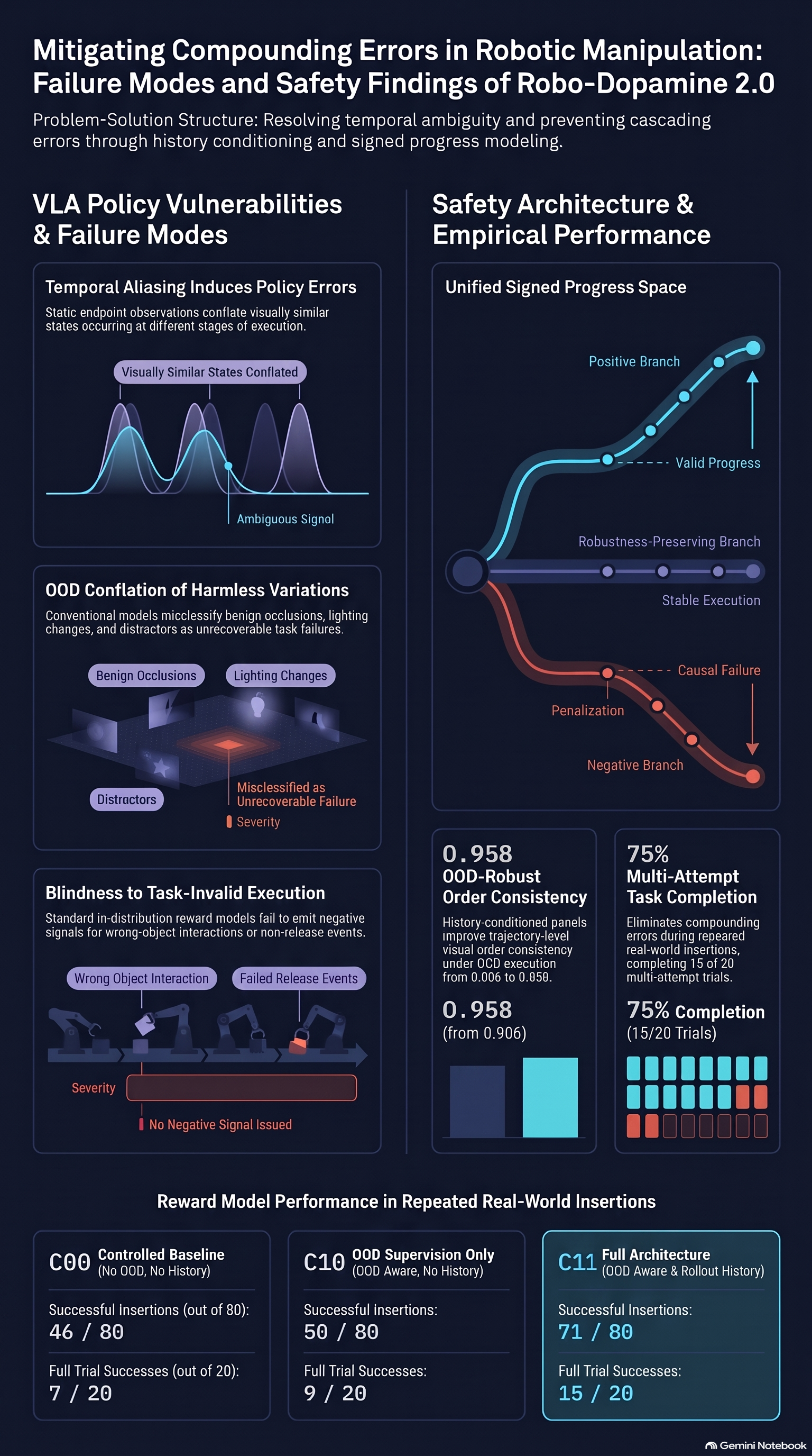
Temporal Ambiguity and Temporal Aliasing: Static frame comparisons struggle to resolve latent progress when visually similar observations correspond to distinct execution phases. These ambiguities often stem from unobserved physical contact events, repeated motion phases, or reordered subgoals where static endpoint observations appear nearly identical despite representing different temporal states.
Weak Out-of-Distribution (OOD) Discrimination: Standard visual reward models often conflate semantics-preserving, benign scene variations with catastrophic, task-invalid failures. While perturbations such as transient visual occlusions, distractor objects, or background shifts ought to preserve progress estimates (robustness), true execution failures—such as empty grasps, wrong-object interactions, or missed object releases—require strict negative reward feedback. In-distribution demonstration datasets rarely contain negative execution states, leaving reward models without explicit supervision to distinguish benign variations from task-invalid failures.

To resolve these challenges, Xu et al. (Aug 2026) introduced Robo-Dopamine 2.0, a history-conditioned and OOD-aware process reward model (PRM). Designed to mitigate compounding errors and off-trajectory policy divergence, Robo-Dopamine 2.0 incorporates temporal context panels and a signed progress representation into a unified pairwise prediction framework. Built upon the Qwen3-VL-8B vision-language backbone and evaluated against prior architectures such as GRM-8B-Pro, Robo-Dopamine 2.0 provides an infrastructure for dense visual credit assignment under off-trajectory and OOD execution.

2. History-Conditioned Pairwise Reward Architecture

Robo-Dopamine 2.0 maintains a pairwise prediction interface while integrating history conditioning to resolve static temporal ambiguity.

Mathematical Formulation

The foundational prediction interface is governed by the General Reward Model (GRM) pairwise progress equation:

$\hat{y}_{ba} = f_\theta(c, R, C_{ba}, X_b, X_a)$

Where:

$c$ represents the textual task instruction.
$R = (r_s, r_g)$ specifies static task-reference anchors corresponding to the task start state ( $r_s$ ) and task goal state ( $r_g$ ).
$C_{ba}$ represents the ordered temporal context frames preceding and separating the queried endpoints.
$(X_b, X_a)$ denotes the ordered pair of queried multi-view endpoint observations, where $X = (x_h, x_l, x_r)$ aggregates canonical view slots: head/third-person camera ( $h$ ), left wrist camera ( $l$ ), and right wrist camera ( $r$ ).
$\hat{y}_{ba}$ represents the predicted signed relative progress.

Temporal Context Structure & Token Budget Trade-offs

The temporal context $C_{ba}$ structures historical frames into two ordered grid layouts:

Pre-query panels ( $M_{1:K}^{pre}$ ): Sampled uniformly from execution states preceding the earlier queried endpoint index ( $W_{pre} = \{t : 0 \le t < \min(t_b, t_a)\}$ ), summarizing historical execution leading into state $X_b$ .
Between-state panels ( $M_{1:L}^{mid}$ ): Sampled uniformly from execution states strictly between the queried endpoints ( $W_{mid} = \{t : \min(t_b, t_a) < t < \max(t_b, t_a)\}$ ), summarizing state transitions separating $X_b$ and $X_a$ .

Images within panels are arranged in standard $3\times3$ grid layouts across canonical camera slots. Missing or unavailable auxiliary views are padded with fixed mask images to maintain structural format consistency.

# Static Baseline Input Layout
I_static = [r_s, r_g, X_b, X_a]

# Robo-Dopamine 2.0 Reference Panel Input Layout
I_ref = [r_s, r_g, M_{1:K}^{pre}, X_b, M_{1:L}^{mid}, X_a]

Ablations conducted by Xu et al. reveal critical engineering trade-offs regarding visual-token capacity. While adding temporal context panels improves visual order consistency, expanding panel grid resolution beyond $3\times3$ (e.g., to $4\times4$ ) or increasing the number of between-state panels ( $B > 2$ ) results in non-monotonic performance degradation. This saturation stems from visual-token budget constraints within the underlying VLM backbone, where excessive context frames dilute attention allocation over key endpoint evidence. Consequently, a $3\times3$ panel layout with $B \in \{1, 2\}$ between-state panels provides the optimal architectural balance.

Context Provenance Contract Across Operational Modes

The provenance of the temporal context frames $C_{ba}$ adapts to the operational query context under a strict provenance contract:

Standard Training Queries: Context panels ( $M_{1:K}^{pre}, M_{1:L}^{mid}$ ) are compiled directly from same-episode expert execution history.
Synthetic OOD Queries: Context panels are compiled exclusively from the unedited, successful source episode, while only the queried endpoints $(X_b, X_a)$ contain the counterfactual OOD edits. This source-only context contract ensures that the reference panels supply nominal, valid execution progress history without obscuring or replacing the edited endpoint evidence.
Online RL Inference: Context panels are constructed dynamically from the agent’s observed rollout history prefix up to rollout step $t$ , requiring no access to expert source trajectories or ground-truth step labels.

Multi-Anchor Online Potential Fusion Mechanism

During closed-loop RL inference, Robo-Dopamine 2.0 evaluates three complementary, normalized query projections at each rollout step $t$ :

$h_\theta(X_b, X_a; C) = \text{clip}\left(\frac{f_\theta(c, R, C, X_b, X_a)}{100}, -1, 1\right)$

Forward-anchored query ( $\hat{h}_t^F$ ): Evaluates progress from the initial rollout observation $X_0$ to the current observation $X_t$ using rollout prefix context $C_t^F$ : $\hat{h}_t^F = h_\theta(X_0, X_t; C_t^F)$
Backward-anchored query ( $\hat{h}_t^B$ ): Evaluates progress from the static goal reference $X_G = r_g$ to current observation $X_t$ without temporal panels: $\hat{h}_t^B = h_\theta(X_G, X_t; \emptyset)$
Incremental query ( $\hat{h}_t^I$ ): Evaluates progress from the immediate previous state $X_{t-1}$ to $X_t$ using step-adjacent rollout context $C_t^I$ : $\hat{h}_t^I = h_\theta(X_{t-1}, X_t; C_t^I)$

Because the initial state $X_0$ possesses a defined potential of zero, a negative forward score operationally signals entry into a task-invalid negative branch. Xu et al. formalize this via a dynamic online branch gate indicator $\hat{b}_t = \mathbb{I}[\hat{h}_t^F < 0]$ (with $\hat{b}_0 = 0$ ). This indicator establishes the query-specific branch floor parameters:

$L_t^F = L_t^B = -\hat{b}_t, \quad L_t^I = -\max\{\hat{b}_{t-1}, \hat{b}_t\}$

To invert normalized signed Hop targets back into potential space, the framework applies the invertibility function $\Gamma(h; \phi, L)$ :

$\Gamma(h; \phi, L) = \begin{cases} \phi + h(1 - \phi), & h \ge 0 \\ \phi + h(\phi - L), & h < 0 \end{cases}$

The individual potential estimates are recovered as: $\hat{\Phi}_t^F = \Gamma(\hat{h}_t^F; 0, L_t^F), \quad \hat{\Phi}_t^B = \Gamma(\hat{h}_t^B; 1, L_t^B), \quad \hat{\Phi}_t^I = \Gamma(\hat{h}_t^I; \hat{\Phi}_{t-1}, L_t^I)$

These three components are aggregated into a unified, context-conditioned online state potential $\hat{\Phi}_t \equiv \hat{\Phi}(\bar{s}_t)$ :

$\hat{\Phi}_t = \text{clip}\left(\frac{\hat{\Phi}_t^F + \hat{\Phi}_t^B + \hat{\Phi}_t^I}{3}, -1, 1\right), \quad \hat{\Phi}_0 = 0$

3. The Signed Progress Space & Counterfactual OOD Pipeline

Mathematical Structure of the Signed Progress Space

Robo-Dopamine 2.0 organizes trajectory states into a continuous signed progress space $\Phi$ , categorizing execution states across positive, robustness-preserving, and negative branches.

Given a successful source trajectory of length $T$ , normalized progress for state index $i \in \{0, \dots, T-1\}$ is defined as $g_i = \frac{i}{T-1}$ . The signed space assigns scalar targets based on state branch classification:

$\Phi(P_i) = g_i \quad \text{(Positive / Valid progress states)}$ $\Phi(R_i) = g_i \quad \text{(Robustness-preserving variations)}$ $\Phi(N_i) = -g_i \quad \text{(Task-invalid negative states, for } i > 0 \text{)}$

Here, positive states ( $P_i$ ) and robustness-preserving states ( $R_i$ ) share identical positive progress values $g_i$ . Task-invalid negative states ( $N_i$ ) are assigned a negative sign with absolute magnitude $|\Phi(N_i)| = g_i$ , indexing failure depth by the source trajectory phase at which the failure occurred.

       [ Positive Branch: Valid Executions (P_i) ] -----> Progress: +g_i
     /
[State] -- [ Robustness Branch: Semantics-Preserving (R_i) ] -> Progress: +g_i
     \
       [ Negative Branch: Task-Invalid Failures (N_i) ] ---> Progress: -g_i

Continuous Signed Hop Target Formulation and Floor Invertibility

For a queried pair $(X_b, X_a)$ with assigned potentials $\phi_b = \Phi(X_b)$ and $\phi_a = \Phi(X_a)$ , the progress differential is explicitly defined as $\Delta_{ba} = \phi_a - \phi_b$ .

To map transitions seamlessly across valid progress, failure, and recovery, the framework incorporates a normalized branch floor parameter:

$L_{ba} = -\max \{ b(X_b), b(X_a) \}$

Where $b(X) \in \{0, 1\}$ is a binary indicator outputting $1$ if state $X$ belongs to a negative branch ( $N$ ), and $0$ otherwise. The Continuous Signed Hop target $H_{ba}$ is formulated as: